online state estimation for a formula student electric car using an unscented kalman filter

17 minutes reading time

How do you measure a vehicle’s velocity when all wheels are driven? The short answer: You can’t. Unless you have big money and can buy one of these. Sadly we didn’t have thousands of euros available to spend on a sensor. So we tried estimating velocity using a cheap IMU, pre-installed motor encoders and some basic signals (e.g. pedal position, brake pressure) that were already available.

As a member of the UPBRacing Team I was responsible for the Vehicle Dynamics sub-team in the season of 2020/2021. In that season we built our first Electric competition car, the PX421E, which built on the rather rudimentary prototype PX212E. The car has four wheel-individual hub motors to provide the highest degree of vehicle dynamics manipulation possible, power of up to 80 kilowatts and weight of around 215 kilos. One thing it didn’t have, though: Proper Torque-Vectoring!

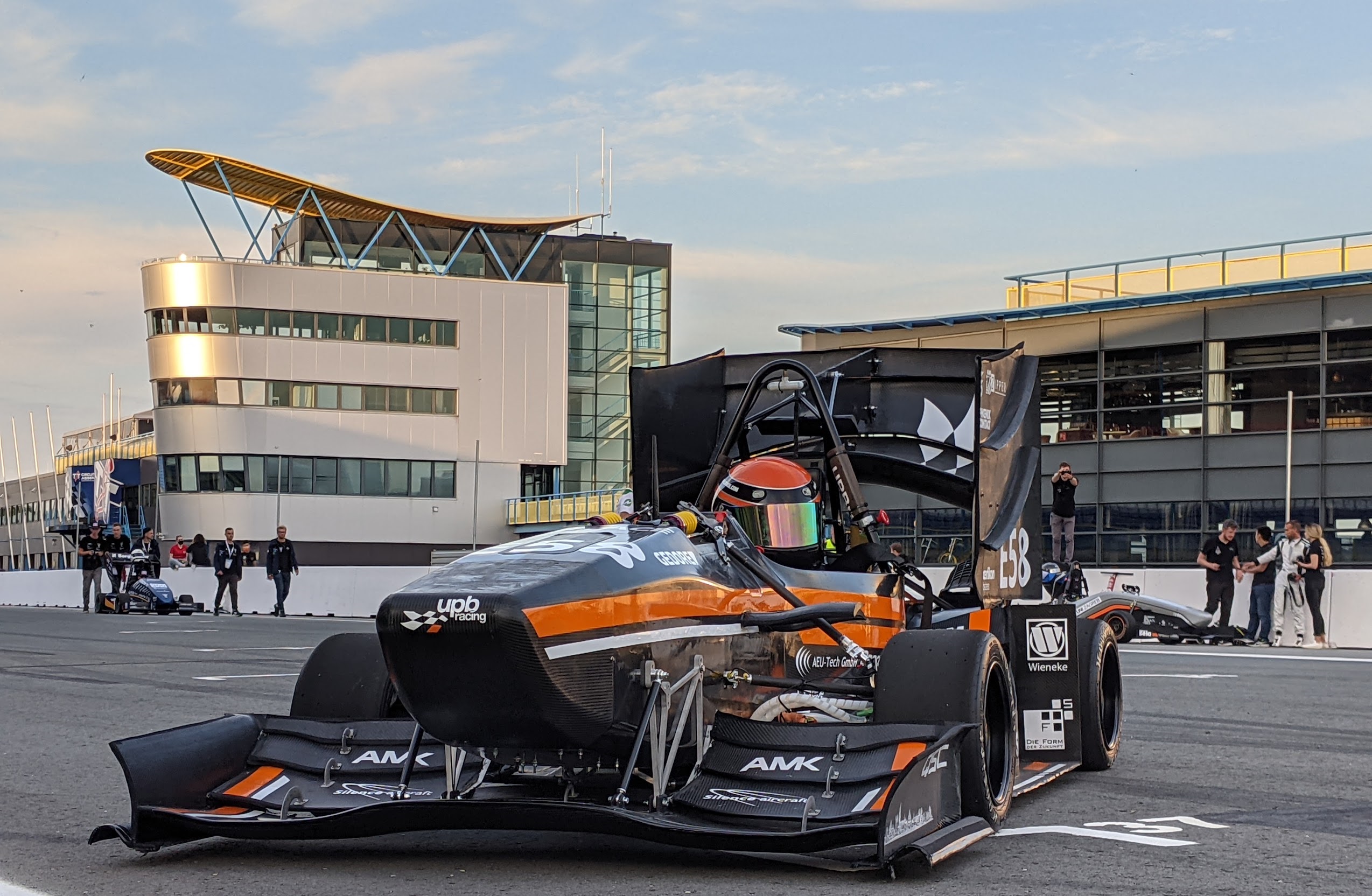PX421E @ TT Circuit Assen

I had already developed a Vehicle Dynamics Control software in my Bachelor’s thesis, but the software was heavily reliant on high-quality vehicle state data. Vehicle velocity being the most important state, as it is used to calculate slip ratios at each wheel. This is fine as long as you have a SIL-environment with all vehicle states available, noise-free. But reality is harsh and we’ve had to realise: One does not simply measure velocity.

In Spring of 2021, I took this challenge as my Master’s project thesis. I ended up implementing an Unscented Kalman Filter (UKF) in MATLAB. The UKF would then (ideally) run in real-time on our ECU, a dSPACE Microautobox III. There was a case for the Extended Kalman Filter (EKF), but from all I’ve read, the UKF is the clear winner over the EKF, bringing non-trivial accuracy and robustness improvements at nearly the same computational cost (Merwe and Wan 2003).

In the following I am not going into details of how Kalman Filters work. I might elaborate on this in the future, but there are great resources available online to get started. To get an intuition on Bayesian probability, you might want to check out Veritasium’s video on Bayes’ theorem. And if you want to understand how Kalman Filters work, I would suggest Roger Labbe’s collection of Jupyter Notebooks on Kalman and Bayesian Filters.

Design and Implementation

The state estimator was implemented as a Square-Root Unscented Kalman Filter (SR-UKF), following the equations of Rudolph Van der Merwe (Merwe and Wan 2003). Compared to the regular UKF, the SR-UKF is said to be computationally more efficient with virtually no difference in accuracy or robustness. While the UKF propagates the state error covariance \(\boldsymbol P_x\) to the next time step, the SR-UKF propagates the square-root \(\boldsymbol S_x \approx \sqrt{\boldsymbol P_x}\) directly, eliminating the need to recalculate square roots in each recursion. For details, see chapter (Merwe and Wan 2003), chapter 3.6.2.

As most modern UKF-implementations do, Merwe’s SR-UKF is utilising the Scaled Unscented Transform (SUT). It provides the filter designer with three parameters, \((\alpha, \beta, \kappa)\) that influence the spread of the Sigma-Points. Sigma-Points, in short, are deterministic sample points whose spread depends to the state error covariance \(\boldsymbol P_x\). For details see (Merwe and Wan 2003).

The design process was as follows:

1. Implement SR-UKF (Merwe and Wan 2003).
2. Verify similar performance to MathWorks’ implementation.
3. Build detailed dual-track vehicle model as reference.
4. Build reduced dual-track vehicle model for real-time use.
5. Evaluate filter performance in several driving scenarios (simulation)
   • Transition from accelerating to hard braking
   • Acceleration with Constant-steer
   • Acceleration with Sine-steer
6. Iterate filter parameters and return to step (5.) until results are satisfactory.
7. Verify robustness against parameter inaccuracies.

First I was going to take the MathWorks implementation of the UKF, but then decided to implement my own version. Theoretically the equations are the same, but while scanning the code of their implementation (yes, it is not protected), I noticed some parts I either didn’t understand or wanted to do differently. It is also easier to debug your software if you have written it yourself (obviously). I did make sure, though, that results were the same with both my own and their implementation.

Just as MathWorks has done, I implemented the equations as a MATLAB class. I tried staying away from Simulink as much as possible and only built a sort of wrapper that ported my MATLAB classes and functions to a Simulink MATLAB-function block. An object-oriented implementation just was a lot easier to work with. It also helped me structure my project in a clean fashion. For generating code directly (or porting it to a Simulink MATLAB-function block), MathWorks also has a guide available.

See my GitHub-repo for source code.

Dual-Track Vehicle Model

Reduced dual-track vehicle model sketch

As noted above, I used two vehicle models to design my filter: A detailed dual-track model and a reduced variant of it. The latter was used inside the SR-UKF to perform predictions and was used to a small extent in the measurement function. It had to be highly computationally-efficient, while still providing all the information we needed. This was probably the hardest task as the filter also had to be efficient enough to run in parallel to the remainder of the ECU’s tasks. The performance of the reference dual-track model didn’t matter really, as the SIL simulations did not have to run in real time. Although long simulation times do eat away at my nerves.

To give you an idea of why a compact system model is important: If we benchmark computational complexity by the size of the loops we encounter each filter iteration the complexity increases quadratically with \(L\), where \(L\) ist the size of the system model’s state vector \(\boldsymbol x\). This is due to the way Sigma Points are determined. In Van der Merwe’s implementation of the SR-UKF, we are determining \(2\cdot L + 1\) Sigma-Points each iteration. Each of these Sigma-Points is propagated through (passed to) the state transition and measurement functions individually. At least that’s how it was in my case, as I wasn’t able to find a way for my dual-track model to take the matrix of Sigma-Points as input.

The reference dual-track model was first implemented in my Bachelor’s thesis as a 3-degrees-of-freedom model (DOF) (translation + yaw). By team effort, we upgraded it to a 6-DOF model as is described in (Schramm et al. 2018), chapter 11.1. Modifications included the drivetrain and tire model. The tire model used is a semi-empirical Magic Formula Tyre 6.1.2 model (Pacejka and Besselink 2012) which was fitted to FSAE TTC data. The state vector \(\boldsymbol x^\text{ref}\) is defined as

with control input \(\boldsymbol u^\text{ref}\)

Not that there are transposed vectors in some rows denoted by \((\circ)^T\). Now, if I haven’t miscounted, you get a whopping 37 elements for \(\boldsymbol x^\text{ref}\). I haven’t actually tried using the UKF with this model, but I imagine performance to be terrible. Remember, the number of major for-loop iterations increase quadratically with the number of states. I reduced the model to the following state vector

and input vector

The first thing I killed were the pose-related states. For my Vehicle Dynamics Control software I did not require the position, though this might be different for a driverless car. And I only need the horizontal velocity, so \(v_z\) was eliminated. Yaw rate is necessary for some kinematic equations, so it was kept. It could have been moved to the control input vector, but that would cause direct feed-through of noise on related states. The same is true for the motor and hydraulic brake torques, but including them in the state vector would increase the size by four states each. In general, I tried to make every signal included in the input vector as clean as possible to noisy filter outputs.

Now, the model from (Schramm et al. 2018) calculates tyre normal forces by modeling of springs, dampers and stabilisers. This way of modeling requires both the Kardan angles we just removed and eight additional states for the vertical deflections of the wheel centerpoints. Great for offline-analysis, bad for online-estimation. In turn, steady-state tyre normal forces were assumed. I have used a modified version of (Heidfeld et al. 2020), which calculates the normal forces from center-of-gravity position and measured accelerations. I did add aerodynamic forces to the equations, because our car has great downforce potential. At least in my simulations this made a huge difference.

As you can also see, the longitudinal and lateral tyre forces are not represented by a state anymore and are instead assumed to be steady-state and passed as an input. This saves eight states, but makes the system model more unstable. But efficiency-wise it was simply not feasible to preserve them.

On a side note, it might have been a great idea to use proprietary vehicle models from big companies to generate reference data. But, after wasting a lot of time on trying to get the existing commercial solution to work, I have developed a fear of bloated engineering software and try to stay away from them as long as possible. Still, a more detailed model would have produced more trustworthy results.

State Transition Function

The state transition function \(\boldsymbol f(\boldsymbol x)\) must have the form

where \(\boldsymbol v_k\) is the process noise and \(p\) are our constant model parameters that our function is initialised with. But our dual-track vehicle model has the form

The easiest solution to this problem is applying Euler-integration to \(\eqref{eq:dualtrack1}\) with sample time \(\tilde{T}\). Assuming additive process noise \(\boldsymbol v_k\), we get

And that would be it — for a pure state estimator. In my case, I upgraded the regular SR-UKF to a Joint SR-UKF. Meaning, I am putting some system parameters inside the state vector which then act as states themselves. If the states correlate with these parameters, you might get a better state estimate. However, don’t expect the parameters to be estimated correctly. They can be thought of as an additional degree of freedom for the filter or, put more plainly, as a garbage collector that compensates for model inaccuracies. As discussed before, this increases the size of the state vector and thereby the computational complexity. It has proven to be a worthy investment, though, as the results were greatly improved.

I added four parameters as states: wheel-individual scaling factors for the tyre friction coefficient. People familiar with the Magic Formula by Pacejka might know of the Scaling Factors denoted by \(\lambda_{(\circ)}\). This sounds fancy, but boils down to a factor multiplied with the model’s tyre friction coefficient \(\mu_{XT}\). The details of this I will spare you, but the complete state vector is an augmented version with \(\boldsymbol x_{p,k}\) being the estimated parameters. You can read on the Joint UKF in (Merwe and Wan 2003) and the scaling factors in (Pacejka and Besselink 2012).

Measurement Function

The measurement function

where \(\boldsymbol n_k\) is the measurement noise, has the following task: transform the state vector into the measurement space. Think about it this way: Imagine we a state estimate \(\hat{\boldsymbol x}\) and a real measurement \(\boldsymbol y\). Assuming we have a function that can calculate a sort of “pseudo-measurement” \(\hat{\boldsymbol y}\) from \(\hat{\boldsymbol x}\), we could compare it to the actual measurement. If our state estimate is good and our measurement can be assumed to be accurate, the difference \(|\hat{\boldsymbol y} - \boldsymbol y|\) should be small. In the simplest case, the “pseude-measurement” \(\hat{\boldsymbol y}\) is the state with (additive) noise and perhaps sensor resolution applied. This is actually the case for the angular wheel velocities and yaw-rate.

Constructing the measurment function is one of the easier tasks when designing Kalman Filters. The only challenge in my case was to infer a pseudo-measurement for the accelerations from the state vector. Note that we also have to account for the IMU not necessarily being placed in the center of gravity. To do this, we can re-use parts of our dual-track model. At some point in this model we are calculating newton’s equation where the acceleration times mass plus the inertia forces is equal to the sum of forces (tires and aero). Then we apply a kinematic transform from the COG to an arbitrary, parametrisable location. Apply sensor resolution (discretisation) and additive noise and we are done here.

While I have implemented my SR-UKF for non-additive noise, where the noise is an input to the system model function \(\tilde{\boldsymbol f}\), I didn’t use it. In fact, I have not yet seen a popular UKF implementation in the literature of vehicle state estimation that makes use of non-additive process (or measurement) noise. I could have probably saved some computation time by implementing the additive-only SR-UKF, but I wasn’t sure what to go for when I started doing my thesis. A use-case for non-additive processs noise I thought of was: Using the already discussed dual-track model form (Schramm et al. 2018), where spring deflections cause tyre normal forces, we could model the “noise” from the road as a deflection imposed from beneath the tire. This would influence the calculations inside \(\tilde{\boldsymbol f}\) and could not simply be “added” onto the state vector. This might be interesting for a filter variant that focuses on tyre load and/or roll/pitch estimation, but could not be applied to my use-case.

Parameter Tuning

After designing the UKF, I had to set the following values

• vehicle parameters (mass, tyre, …)
• SUT parameters (\(\alpha, \beta, \kappa\))
• SR-UKF matrices (\(\boldsymbol R_v, \boldsymbol R_n\))

The vehicle parameters were either taken from CAD (moment of inertia, geometric parameters) or measured with the actual vehicle (e.g. mass). Tyre model parameters were never validated themselves, only fitted to testing data and afterwards slightly modified (accounting for optimal conditions on test-rig).

While I was determining the vehicle parameters, I was painfully aware that most were not completely accurate. Therefore I performed a sensitivity analysis for the most influential parameters. According to my simulations, the UKF was pretty much unconcerned by parameter offsets of up to 20%. The only exception was the effective tyre radius \(r_e\). For \(r_e\) I saw big offsets that increased with parameter imprecision. So assuming a constant tyre radius is not a good idea. Instead I calculated the \(r_e\) using a formula from (Schramm et al. 2018).

The SUT parameters (\(\alpha, \beta, \kappa\)) influence the spread of the Sigma-Points. See the explanation in (Merwe and Wan 2003). For me, the following values have proven themselves.

The most difficult part was setting the covariance matrices (\(\boldsymbol R_v, \boldsymbol R_n\)). Tuning the measurement noise error covariance matrix \(\boldsymbol R_n\) was relatively easy — I just logged the sensor’s measurement in standstill for a long period of time, calculated the variance and then filled the diagonal of \(\boldsymbol R_n\) with said variances. Setting the process noise covariance matrix \(\boldsymbol R_v\) was more difficult. While I get the idea that low values for \(\boldsymbol R_v\) should reduce the filter’s confidence in its predictions, this didn’t help me to find sensible values.

In the end, I tuned \(\boldsymbol R_v\) by a lot of trial-and-error. I could not find a systematic way to set the matrix. If you have lots of measurement data with reference velocity included available, you could perform some curve-fitting-esque optimisation. Most entries on the diagonal ended up being values between \(1\times 10^{-8}\) and \(1\times 10^{-9}\). Only the variance assumed for \(v_x\) was a bit larger: \(1\times 10^{-6}\).

Validation

In December of 2021, our team had the opportunity to borrow a Kistler Correvit sensor from a local company. We could now collect reference velocity data to validate the estimator. Apparently I have been a good boy this year!

Conditions were suboptimal, with temperatures below 6°C and high levels of humidity causing very slippery asphalt. We were forced to switch to rain tires, although the estimator has been designed with a tire model that represents slicks. The results were great anyway, which honestly surprised me. And, to my surprise, I did not have to alter any filter or model parameters!

The Correvit sensor was mounted as shown below, with a non-trivial center-of-gravity offset. This offset has to be considered kinematically to be able to compare the Correvit sensor against the estimator, as the latter estimates velocity in the COG.

Kistler Correvit was placed outside of COG

Denoting the Correvit with \(c\), we have for the measured velocity

where \(\boldsymbol r_c\) is the COG-offset in the vehicle-sketch, \(\boldsymbol v\) the COG-velocity and \(\boldsymbol \omega\) the vector containing roll-, pitch- and yaw-rate. We can rearrange this to

If you write this out and insert \(\omega_x = \omega_y = 0\), you get the velocities that are used in the figures shown. Sadly, we forgot to log the roll- and pitch-rates. So the correction is only accounting for the yaw rate. The COG-offset was estimated only very roughly.

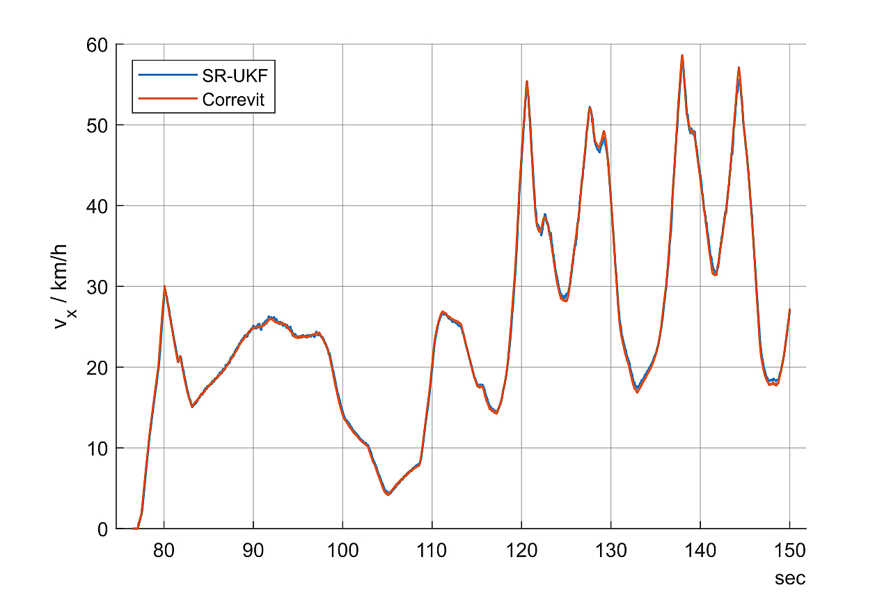
Comparison of longitudinal velocity estimated by SR-UKF and measured by Kistler-Correvit.

In this instance filter performance was great. By the eye only small deviations are visible. Again, I did not include the roll- and pitch-rate in the kinematic transformation. So in reality, they might be slightly higher or lower. To quantify the visual results: We have a standard deviation of \(\sigma = 0.4028\) km/h. Assuming a Gaussian distribution, our the maximum deviation to expect will be \(3\sigma = 1.2084\) km/h. At 100 km/h, that would result in a possible overshoot of about 1.2%. This wouldn’t bother me and is better than I hoped it would be.

Comparison of lateral velocity estimated by SR-UKF and measured by Kistler-Correvit.

The lateral velocity is not as great, although the scale here is much smaller. I did play around with the COG-offset and fictional values for roll- and pitch-rate to see if the offset in \(v_y\) could be explained in a non-sufficient kinematic transformation. And indeed, I was able to improve the visual offset. But without real data, this is not worth much. The standard deviation was about half of what we had for \(v_x\), but keep the different scales in mind. Also, the mounting of the sensor was very basic, consisting of an L-shaped aluminium sheet that could easily bend in the \(y\)-direction through vibrations. This might be partly responsible for the noisy reference signal, as the yaw-rate used for transforming was rather clean.

But not all was as great. Below you will see a section where the filter failed to converge.

“Filter smugness” visible with permanent offset.

We’ve had this issue multiple times actually during testing. Each time this occurred, we had to re-initialise the filter in standstill. Interestingly, the covariance entries of the state error covariance matrix \(\boldsymbol P_x\) remained low. So the SR-UKF “thinks” he is right although he is visibly far off. This is sometimes referred to as filter-smugness. It is very dangerous as it is hard to detect. Usually the UKF will notify you that its estimate is probably not very good with a high covariance for relevant states. But in this case, you have to determine plausibility some other way.

This might happen when the measurement function returns pseudo-measurements very close to the real measurements. Meaning, that for very different states you get very similar measurements and therefore the correction fails. I suspect that the tyre model does not have a large enough negative gradient after the maximum slip has been reached. Therefore the model returns high values of tyre force even at high amounts of slip.

If that was correct, then a solution might have been to modify the tyre model parameters. Another solution could be to increase the process noise covariance matrix and therefore lowering the filter’s confidence in its predictions. Increasing process noise usually also results in higher noise in the final estimate, so I would try that last.

Conclusion

Kalman Filters are cool! I really enjoyed writing my thesis on this topic and I wanted to share this as I expect many teams to struggle with velocity estimation as well. Or rather: I expect many teams to struggle financially like us and therefore must do velocity estimation. Of course, the possible benefits of Kalman Filters to the commercial sector should also be apparent.

I am sure that we can overcome the issues we’ve had with filter-smugness and make the filter more robust and am looking forward to use the SR-UKF to do some advanced Vehicle Dynamics Control. Because when the UKF is working, it is working great!

As a final note: In case you are wondering, the term Unscented has no real meaning. As far as I know, it only means that the UKF does not stink — as in: not as stinky as the EKF.

Update

In April of 2022 we had the opportunity to do more testing with the car. My suspicion that the disappointing validation results for \(v_y\) were rooted in the lack of complete gyroscope data proved to be correct. Applying the same kinematic relationship as in eq. \eqref{eq:relKin}, the results had improved drastically by also considering roll and pitch rates instead of just yaw rate. Also, coordinate-transforming the measured velocities to account for inaccurate sensor mounting improved the results. Using the coordinate transform

where \(\psi\) is the mounting offset angle around the \(Z\)-axis and \(\boldsymbol v^\ast\) the adjusted velocity vector, we can correct the measurements in retrospect. In this case, the angle offset was iteratively set to \(1.2\) degrees.

Validation results for \(v_x\) and \(v_y\) with new data.

Looking at the results here, there are still issues in the lower velocity range. But other than that, we were now very confident in our filter.

Robustness improvements

I wanted to add this update as well, because we were able to successfully address the issues we had with filter smugness, namely velocity getting stuck at zero when starting to drive. We implemented two mechanisms for this:

• Adaptive process noise covariance
• Tuning tyre model parameters

The adaptive process noise covariance was rather simple. In situations where the mean value of all motor angular velocities was low, the diagonal entries of the process noise covariance for \(v_x\) and \(v_y\) were scaled higher. The intention was to make the filter trust its model predictions less at low speeds. This helped a bit on its own, but the real change came from tuning the tyre model parameters.

As we are using a semi-empirical Magic Formula tyre model, we have lots of options to tune the tyre characteristics. However, we were only really interested in tuning PCX1, which mainly affects the slope of the tyre curves after it hits its maximum (minimum). Our reasoning was this: if the filter gets stuck at \(v_x=0\) and instead estimates high slips to reduce the residual between estimated acceleration and measured acceleration, it might be due to the tyre model returning the same longitudinal tyre force (and therefore acceleration) at two different slip ratios. If this is true, setting PCX1 so that the curve were either monotonic or close to monotonicity, the filter could only find one slip ratio which provides an acceleration which is close to the measured one. We played around a bit and in the end got the best results with just setting PCX1 to one.

Effects of PCX1 on tyre characteristics.

We then simulated our Simulink model of the UKF with real logging data from April 2022. Before doing these changes, we would frequently run into described robustness problems at low velocities. After the changes, we did not face this issue once.

Now, one thing we still need to look out for: How does our manipulated tyre model behave at high slip ratios, now that we have eliminated the true maximum and minimum of the curve? We hope that this will not be an issue, because ideally the Vehicle Dynamics Control (VDC) would keep our tyre within its optimal conditions. The VDC still uses the non-manipulated tyre model to calculate the desired slip ratios correctly. If we never reach slip ratios where the estimator tyre model becomes inaccurate, it hopefully becomes a non-issue.

References

1. Merwe R, Wan E (2003) Sigma-Point Kalman Filters for Probabilistic Inference in Dynamic State-Space Models. Proceedings of the Workshop on Advances in Machine Learning
2. Schramm D, Hiller M, Bardini R (2018) Vehicle Dynamics. Springer, Berlin, Heidelberg
3. Pacejka HB, Besselink I (2012) Tire and vehicle dynamics, 3rd ed. Elsevier/BH, Amsterdam and Boston
4. Heidfeld H, Schünemann M, Kasper R (2020) UKF-based State and tire slip estimation for a 4WD electric vehicle. Vehicle System Dynamics 58:1479–1496. https://doi.org/10.1080/00423114.2019.1648836

Last modified on: 28 Jun 2022 23:20. Reason: New data became available.