magic formula tyre library

6 minutes reading time

Today I open-sourced my personal library of Magic Formula Tyre MATLAB functions, which I initially developed as a student working in the Formula Student team UPBracing.

Find source code and packaged library on GitHub!

In the following I will provide an overview of the library and some commentary on the design choices made.

Original Magic Formula

The library is a collection of tools which assisted me as the Vehicle Dynamics Lead in creating, tuning and evaluating Magic Formula Tyre models. Oh, and the functions are all suitable for code-generation and have been used intensively for that purpose in our control and state estimation algorithms. The functions have proven to be quick, accurate and reliable.

As members of the FSAE Tire Test Consortium, we had access to high quality test-bench data of most common Formula Student tyres. Therefore an empirical tyre model made the most sense, considering the relatively fast execution speed with (potential of) very high accuracy (assuming the mode-data-fit is good).

Types and differences between tyre models. Adapted from (Pacejka and Besselink 2012).

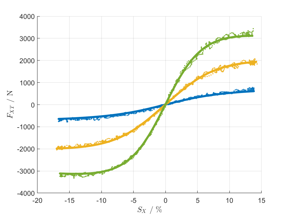
The most popular (semi-)empirical tyre model is the so-called Magic Formula by Hans B. Pacejka. The famous equation has but few parameters but can portray typical tyre behavior accurately.

Where \(y\) would either be \(F_{XT}\) or \(F_{YT}\) and \(x\) would be either slip ratio or slip angle.

For this model, it would be possible to adjust the parameters by hand for a given steady-state condition. However, this would have to be done for every steady-state condition contained in the test-bench data, if accurate model outputs are expected. The found parameters would then have to be implemented in a multidimensional interpolation grid, to enable a fluid transition between these steady-states. This approach, with automated fitting, is taken in this official blog post by MathWorks. The results are lookup-maps for each parameter of the equation.

I find the interpolation approach to be both a bit slow in execution (on real-time hardware) and potentially memory-exhausting. Also, as soon as such interpolation grids have more than 3 dimensions, my brain starts to hurt. And this is what you would need in case you want the parameters to be adaptive to slip ratio, slip angle, inflation pressure and normal load for example. In case you are smarter than me, this might not bother you. But I suggest taking a look at the so-called semi-empirical Magic Formula.

Semi-Empirical Magic Formula

The semi-empirical Magic Formula builds on the Magic Formula introduced before and is, in essence, also a Sine function. However, instead of 4 parameters, the equation(s) now have around 100 parameters to set/fit. Albeit larger, this parameter set does not change depending on the current state of the tire and is also able to portray combined slip conditions (friction ellipse). The incorporation of the so-called Similarity Method, which enables the equations to even extrapolate tyre behaviour across tested steady-state conditions, and considering physical limitations of tyres expressed in the form of adapted equations, gave the model the attribute of being semi-empirical. (Pacejka and Besselink 2012) In the following, the semi-empirical Magic Formula will just be referred to as the Magic Formula.

All of this has the advantage of more efficient execution and less memory consumed on the target hardware. However, it is also much more difficult to tune, but not as difficult as it might seem at first. In practice, most of these parameters are just set to either zero or unity, as a great model fit can be achieved with only a fraction of these parameters.

In any case, it is probably not something you would want to tune by hand, apart from fine-tuning the fitted parameter set. The Magic Formula Tyre equations, in completion, are found in chapter 4.3.2 of (Pacejka and Besselink 2012). Pacejka also provides in-depth explanations of the equations, in case you are interested. The book should be freely available with most student VPNs as PDF. The official Magic Formula Tyre/MF-Swift 6.2 manual is a great addition to Pacejka’s book as it provides brief descriptions of each parameter and its function.

Implementing Magic Formula Tyre

Finding implementations of Magic Formula Tyre that are open-sourced and non-commercial is difficult. There is MFeval, but in my experience it was too slow to be useful in real-time applications and offline fitting operations. The cause appeared to be excessive use of for-loops instead of more efficient matrix operations. I ended up building my own implementation.

Peeking into the code, the implementation of the equations is pretty straight-forward. Simply translate math into code. Have the Pacejka book on one half of your monitor, the MATLAB editor on the other half. You can then write the equations neatly line by line. This process is very prone to mistyping, though, be warned!

function Fx0 = Fx0(p,longslip,inclangl,pressure,Fz)
% (4.E1)
FNOMIN = p.FNOMIN.*p.LFZO;

% (4.E2a) 
dfz = (Fz-FNOMIN)./FNOMIN;

% (4.E2b) 
dpi = (pressure-p.NOMPRES)./p.NOMPRES;

% (4.E11) 
Cx = p.PCX1.*p.LCX;
...

end

One difficult question is: How are parameter names decided to be understandable and perhaps even standardized? Thankfully, we have the official Magic Formula Tyre/MF-Swift 6.2 manual to our aid. It includes the variable names and descriptions for all Magic Formula Tyre (and MF-Swift) parameters. I used those definitions to establish my parameter names, which makes the Magic Formula Tyre manual a useful document when working with the library. To illustrate, \(p_{Cy1}\) in the book becomes PCY1 in MATLAB code. The visible similarity allows for easy matching of literature and the implementation.

Another question: How to we create parameter sets? I wanted to avoid a long script of a struct being written to, line by line. I felt a cleaner way of doing things was to implement a MATLAB class for a parameter set. This would later also become beneficial to creating a fitting algorithm and potential GUIs built around the library. The class initializes the parameter set with sensible values (if possible a-priori) and min/max values recommended in Pacejka’s book. The min/max values can used by the user as reference, but also provide functional use in automated curve-fitting applications.

classdef Parameters
    properties
        %% [MODEL]
        FITTYP    = magicformula.v62.Parameter(62,'Magic Formula version number')
        TYRESIDE  = magicformula.v62.Parameter('LEFT','Position of tyre during measurements')
        LONGVL    = magicformula.v62.Parameter([], 'Reference speed')
        ...
        %% [LATERAL_COEFFICIENTS]
        PCY1      = magicformula.v62.ParameterFittable(1.9, 1.5, 2, 'Shape factor Cfy for lateral forces')
        PDY1      = magicformula.v62.ParameterFittable(0.8, 0.1, 5, 'Lateral friction Muy')
        PDY2      = magicformula.v62.ParameterFittable(-0.05, -0.5, 0, 'Variation of friction Muy with load')
        ...
end

The parameter descriptions were also taken from the Magic Formula Tyre manual. To use this parameter set for calculating the tyre forces, a conversion to struct was required first. Technically, a class object can also be used as an input argument to the equations, but ultimately code-generation would make this an awkward solution, so a standard data type like structs seemed more appropriate. The conversion is easily done by calling the struct() method on the Parameters object. By using function overloading, we can change the behaviour of the struct() function exclusively for Parameters objects.

Finally, all equations culminate in the magicformula.v62.eval() function, which calculates the tyre forces \(F_{XT}\) and \(F_{YT}\) in wheel-fixed coordinates from varying inputs (slip angle, slip ratio, normal load, …) and a given parameter set. The difficult process obviously is acquiring a fitted parameter set for the tyre of interest. But once you have it, the evaluation of the model is a one-liner.

[Fx,Fy] = magicformula.v62.eval(p,slipangl,longslip,inclangl,inflpres,FZW,tyreSide)

Other Features

The library also comes with functions to read from and write to .tir (Tyre Property File) files, which is a common file standard for exchanging tyre model parameters with commercial software. In Formula Student I made use of this package to export my parameter set to be used in a Siemens NX Multibody simulation. See the +tir package of the library or use the convenience methods of the magicformula.v62.Model class.

Additionally, a fitting-framework is provides which largely automates tyre model creation from measurement data. See the magicformula.v62.Fitter class and the +tydex package. The latter provides an in-memory representation of test-bench data to be used by the magicformula.v62.Fitter class. Note: In case you are trying to model Formula Student tyres, I have already written a parser that separates the time-series data into steady-states. See folder +tydex/+parsers/.

I might elaborate on these features in another post, but documentation will be added to the GitHub repository in any case.

Edit: I also developed a GUI application for fitting semi-empirical Magic Formula models to data. It has been featured on the Student Lounge of MathWorks. Read about it here.

References

1. Pacejka HB, Besselink I (2012) Tire and vehicle dynamics, 3rd ed. Elsevier/BH, Amsterdam and Boston

Last modified on: 29 Jun 2022 00:18. Reason: SEO optimization.